
Consumer and Producer Surplus on a Supply and Demand Graph
A ticket buyer who was willing to pay more than the ticket price gains from the purchase. A seller who would have accepted less gains too. A surplus graph adds up those gains across a market. It also shows what changes when a price rule or tax prevents some trades.
For background, see how to find equilibrium, how to read the axes, and what shifts a curve in the graph maker.
Where to shade consumer and producer surplus
Consumer surplus (CS) is what buyers were willing to pay minus what they actually paid. For each unit sold, the demand curve gives the buyer’s willingness to pay. Shade the area below demand and above the price buyers pay, stopping at the quantity actually traded.
Producer surplus (PS) is what sellers receive minus the minimum they would accept for the units they sold. Each point on the supply curve gives the cost of supplying that unit in this model. Shade above supply and below the price sellers receive. Producer surplus measures gains above variable costs. A business may still have fixed costs to cover.
The horizontal width of a shaded region is measured in units. Its height is measured in dollars per unit, so the area is in dollars. When the height falls linearly to zero, use a triangle. If both ends have a positive height, use a trapezoid by multiplying the width by the average of the two heights.
Competitive equilibrium
Consider a market for tickets to a school event, with price P in dollars and quantity in tickets. Suppose Qd = 120 − 3P, Qs = 2P − 10. The highest willingness to pay is $40, and the supply curve begins at $5.
Setting demand equal to supply gives P = (120 + 10) ÷ (3 + 2) = $26. Substituting gives Q = 120 − 3 × 26 = 42 tickets.
The consumer triangle is 42 × (40 − 26) ÷ 2 = $294. The producer triangle is 42 × (26 − 5) ÷ 2 = $441. Their sum is $735.
At the last ticket sold, willingness to pay and the cost of supplying the ticket are equal. Earlier tickets create positive gains. That shrinking gap explains why both shaded areas taper to a point.
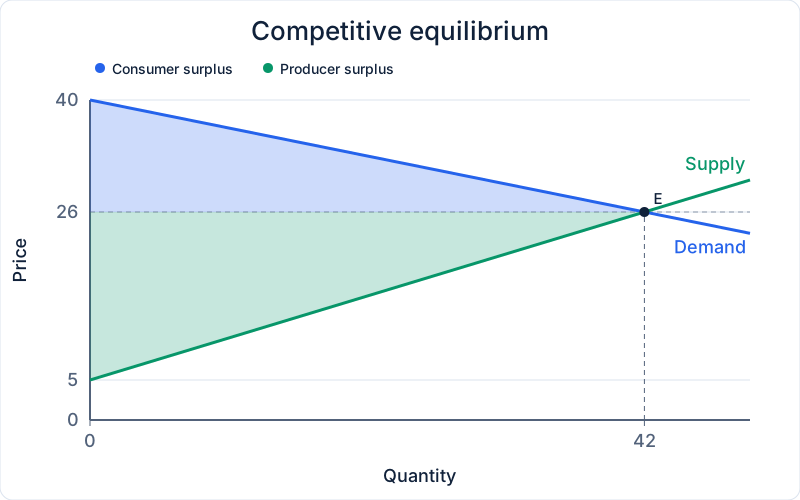
Make this graph in the Supply and Demand Graph Maker. Open Generate from linear equations and enter the market equations to plot the curves, then use the shaded example as a reference.
Price ceiling
Set a maximum price of $20. Buyers want 60 tickets, but sellers offer 30. The shortage is 60 − 30 = 30 tickets. Assume the buyers willing to pay the most get the available tickets, with no waiting costs or resale.
At the last ticket sold, the buyer’s willingness to pay is $30. That leaves a positive height above the ceiling at the right edge of the blue area. Consumer surplus is a trapezoid. Seller surplus is a triangle because the cost of the last ticket equals the ceiling.
Some buyers who still get tickets gain from the lower price. Buyers shut out of the market lose the chance to trade. That is why a lower price on its own cannot tell you whether buyers as a group gain. If tickets go to buyers by lottery or queue, the result can differ from this example.
CS = 30 × (20 + 10) ÷ 2 = $450. PS = 30 × (15 + 0) ÷ 2 = $225. The deadweight loss (DWL) triangle runs from 30 to 42 tickets. Its area is 12 × (10 + 0) ÷ 2 = $60.
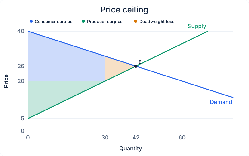
Make this graph in the Supply and Demand Graph Maker. Open Generate from linear equations and enter the market equations to plot the curves, then use the shaded example as a reference.
Price floor
Set a minimum price of $32. Sellers offer 54 tickets, and buyers want 24. The excess supply is 54 − 24 = 30 tickets. Assume the lowest-cost sellers make the sales and nobody buys the excess.
At the last ticket sold, the producer’s cost is $17, below the floor, so the green area ends with positive height. Producer surplus is a trapezoid. Consumer surplus is a triangle because the last buyer’s willingness to pay equals the floor.
A higher price helps the sellers who still make a sale, while others sell nothing. The graph counts gains from actual sales. If a government bought the unsold tickets, its spending and any value from those purchases would need to be included in a different calculation.
CS = 24 × (8 + 0) ÷ 2 = $96. PS = 24 × (27 + 15) ÷ 2 = $504. The deadweight loss (DWL) triangle runs from 24 to 42 tickets. Its area is 18 × (15 + 0) ÷ 2 = $135.
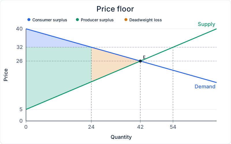
Make this graph in the Supply and Demand Graph Maker. Open Generate from linear equations and enter the market equations to plot the curves, then use the shaded example as a reference.
Per-unit tax
Now remove the price rules and charge $10 per ticket. The buyer price equals the seller price plus the tax. Substituting that relationship into the demand equation and setting it equal to supply gives a seller price of $20, a buyer price of $30, and 30 tickets sold.
The buyer price rose by $4 from the original price, and the seller price fell by $6. Buyers bear 40% of the tax per unit and sellers bear 60%. This follows from the prices each side faces even if one side sends the entire tax payment to the government.
Tax revenue is the rectangle between the two prices, 30 × $10 = $300. Its width covers every unit still traded. The triangle of forgone gains begins where that rectangle ends.
CS = 30 × (10 + 0) ÷ 2 = $150. PS = 30 × (15 + 0) ÷ 2 = $225. The deadweight loss (DWL) triangle runs from 30 to 42 tickets. Its area is 12 × (10 + 0) ÷ 2 = $60.
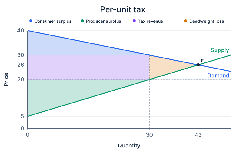
Make this graph in the Supply and Demand Graph Maker. Open Generate from linear equations and enter the market equations to plot the curves, then use the shaded example as a reference.
Compare the four outcomes
Total surplus adds consumer and producer surplus plus government revenue. Deadweight loss tells you how far that total falls below the competitive result. Add it back as a check against the original total in each row. Payments transferred between people affect who gains, while lost trades shrink the total.
| Scenario | CS | PS | Revenue | DWL | Total surplus |
|---|---|---|---|---|---|
| Competitive equilibrium | $294 | $441 | $0 | $0 | $735 |
| Price ceiling | $450 | $225 | $0 | $60 | $675 |
| Price floor | $96 | $504 | $0 | $135 | $600 |
| Per-unit tax | $150 | $225 | $300 | $60 | $675 |
Common mistakes when shading surplus
- Use the actual quantity traded. A ceiling can make buyers want more than sellers offer. A floor can make sellers offer more than buyers want. End the surplus areas at the smaller quantity.
- Use the price each side faces. With a tax, measure buyer surplus above the buyer price and seller surplus below the seller price. Using one price for both puts some of the revenue rectangle into private surplus.
- Start DWL at the last unit traded. The triangle is between the curves on the side toward the original equilibrium quantity. Shading to the left would include units that still sell.
- Check the shape before using a formula. A surplus area can have a nonzero height at both ends. The triangle shortcut only works when one end reaches zero.
Practice with a different market
Use Qd = 96 − 2P, Qs = 4P − 24 for a market for notebooks. Start from the competitive graph, then apply each policy separately. Use the same buyer and seller selection assumptions as in the ticket examples. Sketch the shaded areas before opening the answers.
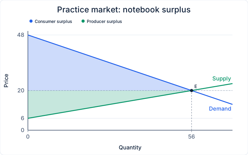
Find the competitive price, quantity, and both surplus areas.
The price is $20 and 56 units trade. CS = 56 × (28 + 0) ÷ 2 = $784. PS = 56 × (14 + 0) ÷ 2 = $392.
At a $16 ceiling, what is the shortage and how much surplus is lost?
The shortage is 64 − 40 = 24 units. DWL = 16 × (12 + 0) ÷ 2 = $96.
At a $24 floor, how many units go unsold and what is seller surplus?
Excess supply is 72 − 48 = 24 units. With the lowest-cost sellers trading, PS = 48 × (18 + 6) ÷ 2 = $576.
With a $6 per-unit tax, what prices do buyers and sellers face, and who pays more?
Buyers pay $24 and sellers keep $18. Buyers bear $4 per unit and sellers bear $2. Revenue is $288, and DWL is $24.
Make this graph in the Supply and Demand Graph Maker and check how your curves compare with the practice chart.